Linear Regression and Clustering
library(tidyverse)
library(dplyr)
library(car)
library(modelr)
library(mgcv)
library(patchwork)
library(factoextra)
Introduction
After our EDA and statistical analysis, we consider to generate a linear regression to better express the relationship between Life Expectancy and other variables. In particular, we set une_life as our response variable and we only look at the year of 2015.
Dataset Preparation
In the beginnig, to prepare our dataset for multiple linear regression, we delete mortality related variables, delete une_pop, which is not a good predictor of life expenctancy, and also delete variables that have high correlation values presented in EDA section. Specifically, we use “measles” to be the representative of vaccination variables–hepatitis, measles, polio, and diphtheria. Moreover, we use “bmi” to be another representative of age5_19thinness, age5_19obesity, and bmi.
In the end, we limit the data to year 2015, and set the Income Reference Group to Low Income.
data <-
  read_csv("data/Merged_expectation.csv") %>%
  filter(year == 2015) %>%
  select(alcohol:percent_w_in_lower_house) %>%
  select(-hepatitis, -polio, -diphtheria, -age5_19thinness, -age5_19obesity, -une_infant, -une_pop) %>%
  mutate(income_group = as.factor(income_group),
         income_group = relevel(income_group, ref = "Low income"))
Model 1
First, we look at the number of missing data we have on each column, at year 2015. The table below shows variables that have less than 5% NA’s.
NA_table_1 <- data %>%
  is.na() %>%
  colSums()
NA_table_1[NA_table_1 <= 10] %>%
knitr::kable(col.names = c("Counts of NA"))| Counts of NA | |
|---|---|
| alcohol | 1 |
| bmi | 2 |
| measles | 0 |
| basic_water | 0 |
| gghe_d | 6 |
| che_gdp | 7 |
| une_life | 0 |
| une_gni | 7 |
| PM_value | 0 |
| income_group | 1 |
| Developed / Developing Countries | 0 |
| percent_w_in_lower_house | 5 |
Limited to the variables that we have less than 5% NA’s (which is less than 10 NAs), also exclude variables that have high correlation value, we could generate our first basic linear model, with selected variables of alcohol, bmi, measles, basic_water, che_gdp (health expenditure per gdp, gghe_d is deleted since it represents similar aspects), une_gni, PM_value, income_group (Developed/Developing Countries is deleted since it is similar to income_group), percent_w_in_lower_house, and our response variable of une_life.
- Model 1: une_life ~ alcohol + bmi + measles + basic_water + che_gdp + une_gni + PM_value + income_group * percent_w_in_lower_house
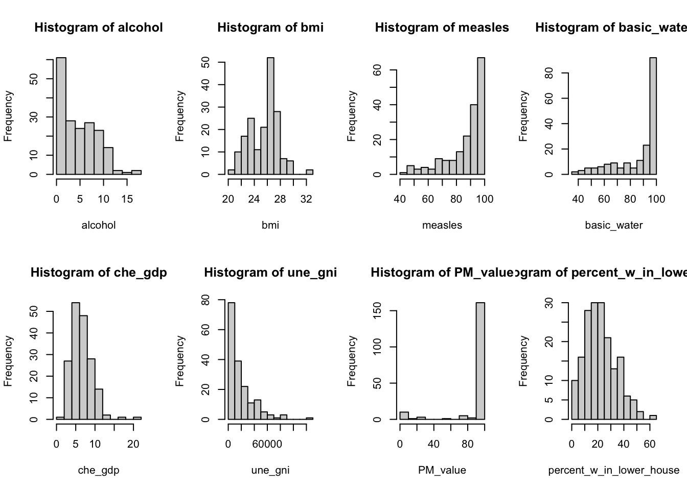
The following table shows the distribution of all numerical variables here.
colname <- c("alcohol", "bmi", "measles", "basic_water", "che_gdp", "une_gni", "PM_value", "percent_w_in_lower_house")
par(mfrow=c(2, 4))
data_1_a <- data.frame(data)
for (i in 1:8) {
  variable <- data_1_a[colname[i]][ ,1]
  hist(variable, main = paste("Histogram of", colname[i], sep = " "), xlab = colname[i])
}
Delete all the NA rows in the data, consider intersection between income_group and percent_w_in_lower_house, using step function with backwards direction. Then we generate our first model.
# delete all the Na columns
data_1 <- data %>%
  select(une_life, alcohol, bmi, measles, basic_water, che_gdp, une_gni, PM_value, income_group, percent_w_in_lower_house) %>%
  drop_na()
# fit the model one
m <- lm(une_life ~ alcohol + bmi + measles + basic_water + che_gdp + une_gni + PM_value + income_group * percent_w_in_lower_house, data = data_1)
# use stepwise function
m1 <- step(m, direction = "backward", trace = FALSE)# create table for regression output
m1 %>%
summary() %>%
broom::tidy() %>%
select(term, estimate, p.value) %>%
knitr::kable(
caption = "Estimate and P-value of Model 1 for Year 2015 Life Expectancy (Income Reference Group is Low Income)",
col.names = c("Predictor", "Estimate", "P-value"),
digits = 3
)| Predictor | Estimate | P-value |
|---|---|---|
| (Intercept) | 37.297 | 0.000 |
| alcohol | -0.164 | 0.102 |
| measles | 0.066 | 0.035 |
| basic_water | 0.271 | 0.000 |
| income_groupHigh income | 6.368 | 0.009 |
| income_groupLower middle income | 3.437 | 0.068 |
| income_groupUpper middle income | 4.358 | 0.065 |
| percent_w_in_lower_house | 0.156 | 0.012 |
| income_groupHigh income:percent_w_in_lower_house | -0.003 | 0.973 |
| income_groupLower middle income:percent_w_in_lower_house | -0.151 | 0.041 |
| income_groupUpper middle income:percent_w_in_lower_house | -0.152 | 0.054 |
From the above, variables like bmi, che_gdp, une_gni, PM_value are deleted according to backwards step function. One way to explain this is that these variables have high correlation with income_group–in higher income countries(une_gni), people have more access to healthy foods and healthy life styles (bmi), governments also spend more money on public health(che_gdp), as well as on building a clean environment(PM_value).
From the estimates, we can conclude that, increase of alcohol consumption has negative effects on life expectancy. Increasing access to vaccines and clean water, the empowerment of women, and higher income will lead to a longer life.
Another thing that needs to be aware of is that the intersection of income group and women in parliament(percent_w_in_lower_house). The variable percent_w_in_lower_house is significant itself, but it is more significant in middle income and upper income groups. In other words, after a country reaches a certain level of income, increasing women’s voice in the country actually helps people live longer, which follows the intention that we chose to include this variable in the first place. (Since 0.156 - 0.152 > 0, keeping other variables constant, percent_w_in_lower_house increases, the predicted life expectancy will increase.)
The model 1’s R-adjusted score reaches 0.7808107.
Below are the analysis plots of the model. These plot shows that the residuals are normally distributed, independent, but may not have a constant variance–it has a linear trend in the end according to the third plot. In second plot, the points follows the line, so the regression function is linear. Therefore, maybe we don’t need to add transformation to our response variable.
par(mfrow=c(2,2))
plot(m1)
- The final Model 1 is une_life ~ alcohol + measles + basic_water + income_group * percent_w_in_lower_house
Model 2
Second, we only look at the countries with existing une_literacy data and found out the number of NA in other variables of these countries, at year 2015. The table below shows variables that have less than 5% NA’s.
NA_table_2 <- data %>%
  filter(is.na(une_literacy) == FALSE) %>%
  is.na() %>%
  colSums()
NA_table_2[NA_table_2 <= 3] %>%
knitr::kable(col.names = c("Counts of NA"))| Counts of NA | |
|---|---|
| alcohol | 0 |
| bmi | 0 |
| measles | 0 |
| basic_water | 0 |
| gghe_d | 0 |
| che_gdp | 0 |
| une_life | 0 |
| une_gni | 1 |
| une_literacy | 0 |
| PM_value | 0 |
| income_group | 1 |
| Developed / Developing Countries | 0 |
| percent_w_in_lower_house | 2 |
Here, limited to the variable that we have less than 5% NA’s (which is less than 3 NAs), also exclude variables that have high correlation value, we could generate our second basic linear model, with selected variables of alcohol, bmi, measles, basic_water, che_gdp, une_gni, une_literacy, PM_value, income_group, percent_w_in_lower_house, and our response variable of une_life.
- Model 2: une_life ~ alcohol + bmi + measles + basic_water + che_gdp + une_gni + une_literacy + PM_value + income_group + percent_w_in_lower_house + income_group * percent_w_in_lower_house
(Also consider intersection here)
The following table shows the distribution of all numerical variables here.
# delete all the Na columns, and limit to countries with existing une_literacy data
data_2 <- data %>%
  filter(is.na(une_literacy) == FALSE) %>%
  select(une_life, alcohol, bmi, measles, basic_water, che_gdp, une_gni, une_literacy, PM_value, income_group, percent_w_in_lower_house) %>%
  drop_na()
colname <- c("alcohol", "bmi", "measles", "basic_water", "che_gdp", "une_gni", "une_literacy", "PM_value", "percent_w_in_lower_house")
par(mfrow=c(3, 3))
data_2_a <- data.frame(data_2)
for (i in 1:9) {
variable <- data_2_a[colname[i]][ ,1]
hist(variable, main = paste("Histogram of", colname[i], sep = " "), xlab = colname[i])
}
Delete all the NA rows in the data, consider intersection between income_group and percent_w_in_lower_house, using step function with backwards direction. Then we generate our second model.
# fit the model two
m <- lm(une_life ~ alcohol + bmi + measles + basic_water + che_gdp + une_gni + une_literacy + PM_value + income_group * percent_w_in_lower_house, data = data_2)
# use stepwise function
m2 <- step(m, direction = "backward", trace = FALSE)
# create table for regression output
m2 %>%
summary() %>%
broom::tidy() %>%
select(term, estimate, p.value) %>%
knitr::kable(
caption = "Estimate and P-value of Model 2 for Year 2015 Life Expectancy Only in Countries With Existing Literacy Data",
col.names = c("Predictor", "Estimate", "P-value"),
digits = 3
)| Predictor | Estimate | P-value |
|---|---|---|
| (Intercept) | 48.798 | 0.000 |
| bmi | -0.521 | 0.126 |
| measles | 0.102 | 0.100 |
| basic_water | 0.185 | 0.002 |
| che_gdp | 0.464 | 0.088 |
| income_groupHigh income | 13.186 | 0.000 |
| income_groupLower middle income | 6.742 | 0.005 |
| income_groupUpper middle income | 8.695 | 0.002 |
From the above, variables like alcohol, une_gni, une_literacy, PM_value, income_group:percent_w_in_lower_houseare, percent_w_in_lower_houseare are deleted according to backwards step function. It is very different from the model 1 when we limit to 37 countries. Moreover, even though we specifically make sure every country has literacy data, literacy is not significant enough to be included in the linear regression model.
The intersection of income group and women in parliament(percent_w_in_lower_house) is also been deleted. Therefore, we can conclude that the model we generate in a small range of countries with complete literacy data entries is very different from the model generated from a larger dataset, while literacy data is not significant in the small range of countries. To conclude, we should discard literacy variable, and also discard model 2.
The model 2’s R-adjusted score reaches 0.857607. This is reasonable, since we generate model 2 in a small range of countries.
- Therefore, we should discard literacy variable, and also discard model 2. We should consider Model 1 as a great subset of the full model.
Compare Model 1 with Full Model
Full Model is the Year 2015 full dataset except mortality rate and except variables with more than 5% NAs.
- Full Model: uni_life ~ hepatitis + polio + diphtheria + age5_19thinness + age5_19obesity + une_pop + alcohol + bmi + measles + basic_water + gghe_d + che_gdp + une_pop + une_gni + PM_value + income_group + percent_w_in_lower_house + Developed/Developing Countries
# generate the Year 2015 full dataset except mortality rate
data_full <-
  read_csv("data/Merged_expectation.csv") %>%
  filter(year == 2015) %>%
  select(une_life, hepatitis, polio, diphtheria, age5_19thinness, age5_19obesity, une_pop , alcohol, bmi, measles, basic_water, gghe_d, che_gdp, une_pop, une_gni, PM_value, income_group, percent_w_in_lower_house, `Developed / Developing Countries`) %>%
  drop_na()
m_full <- lm(une_life ~ ., data = data_full)
m1 %>%
summary() %>%
broom::glance() %>%
bind_rows(summary(m_full) %>% broom::glance()) %>%
mutate(model = c("Model 1", "Full Model")) %>%
select(model, everything()) %>%
knitr::kable(
caption = "Comparision of Model 1 and Full Model",
digits = 3
)| model | r.squared | adj.r.squared | sigma | statistic | p.value | df | df.residual | nobs |
|---|---|---|---|---|---|---|---|---|
| Model 1 | 0.794 | 0.781 | 3.693 | 59.777 | 0 | 10 | 155 | 166 |
| Full Model | 0.817 | 0.791 | 3.541 | 31.710 | 0 | 19 | 135 | 155 |
From the above table, Model 1 and Full Model do not have big difference on adjusted R^2, but Model 1 has less predictors, which is much better.
Transformation on Response Variable of Model 1
First, we want to find whether response variable une_life needs transformation.
inverseResponsePlot(m1, key = TRUE)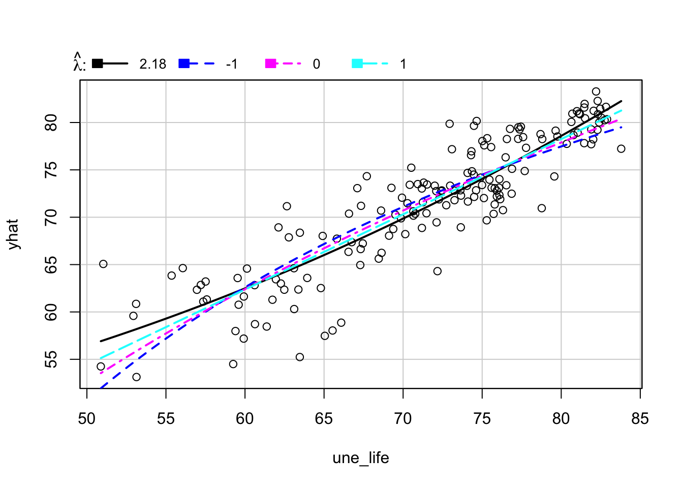
##     lambda      RSS
## 1  2.17794 1637.306
## 2 -1.00000 1953.745
## 3  0.00000 1782.892
## 4  1.00000 1678.616
From the above plot, the best \(\lambda\) for model 1 is 2.17794, which is different from 1. Therefore, we will apply \(\lambda\) equal to 2.17794 to une_life.
# Fit model 1 with une_life^2.17794
m1_tr <- lm((une_life)^2.17794 ~ alcohol + measles + basic_water + income_group * percent_w_in_lower_house, data = data_1)
# create table for regression output
m1_tr %>%
  summary() %>%
  broom::tidy() %>%
  select(term, estimate, p.value) %>%
  knitr::kable(
      caption = "Estimate and P-value of Transformed Model 1 for Year 2015 Life Expectancy",
      col.names = c("Predictor", "Estimate", "P-value"),
      digits = 3
)| Predictor | Estimate | P-value |
|---|---|---|
| (Intercept) | 695.168 | 0.403 |
| alcohol | -52.404 | 0.099 |
| measles | 19.506 | 0.047 |
| basic_water | 82.789 | 0.000 |
| income_groupHigh income | 1960.037 | 0.011 |
| income_groupLower middle income | 942.528 | 0.112 |
| income_groupUpper middle income | 1248.515 | 0.093 |
| percent_w_in_lower_house | 43.753 | 0.025 |
| income_groupHigh income:percent_w_in_lower_house | 12.999 | 0.603 |
| income_groupLower middle income:percent_w_in_lower_house | -42.804 | 0.065 |
| income_groupUpper middle income:percent_w_in_lower_house | -41.973 | 0.091 |
The transformed model 1’s R-adjusted score reaches 0.7886281. The adjusted R square increases ~0.01 after transformation, which is close to the adjusted R square of the full model. However, while the difference of adjusted R square is small, for better interpretation, we decide to choose the original Model 1.
Finally, our linear regression model on life expectancy is une_life ~ alcohol + measles + basic_water + income_group * percent_w_in_lower_house.
Cross Validation
- Model: une_life ~ alcohol + measles + basic_water + income_group * percent_w_in_lower_house.
We divides the Year 2015 dataset to train ans test two datasets 100 times. The graph below shows RMSE distribution in test datasets.
# generate a cv dataframe
cv_df <-
  crossv_mc(data_1, 100) %>%
  mutate(
    train = map(train, as_tibble),
    test = map(test, as_tibble))
# fit the model to the generated CV dataframe
cv_df <-
  cv_df %>%
  mutate(
    model  = map(train, ~lm(une_life ~ alcohol + measles + basic_water + income_group * percent_w_in_lower_house, data = .x)),
    rmse = map2_dbl(model, test, ~rmse(model = .x, data = .y)))
# plot the prediction error
cv_df %>%
  select(rmse) %>%
  pivot_longer(
    everything(),
    names_to = "model",
    values_to = "rmse") %>%
  ggplot(aes(x= model, y = rmse)) +
  geom_violin() +
  labs(
    title = "Prediction Errors For Our Model Under CV",
    x = "Model 1",
    y = "Prediction Errors"
) 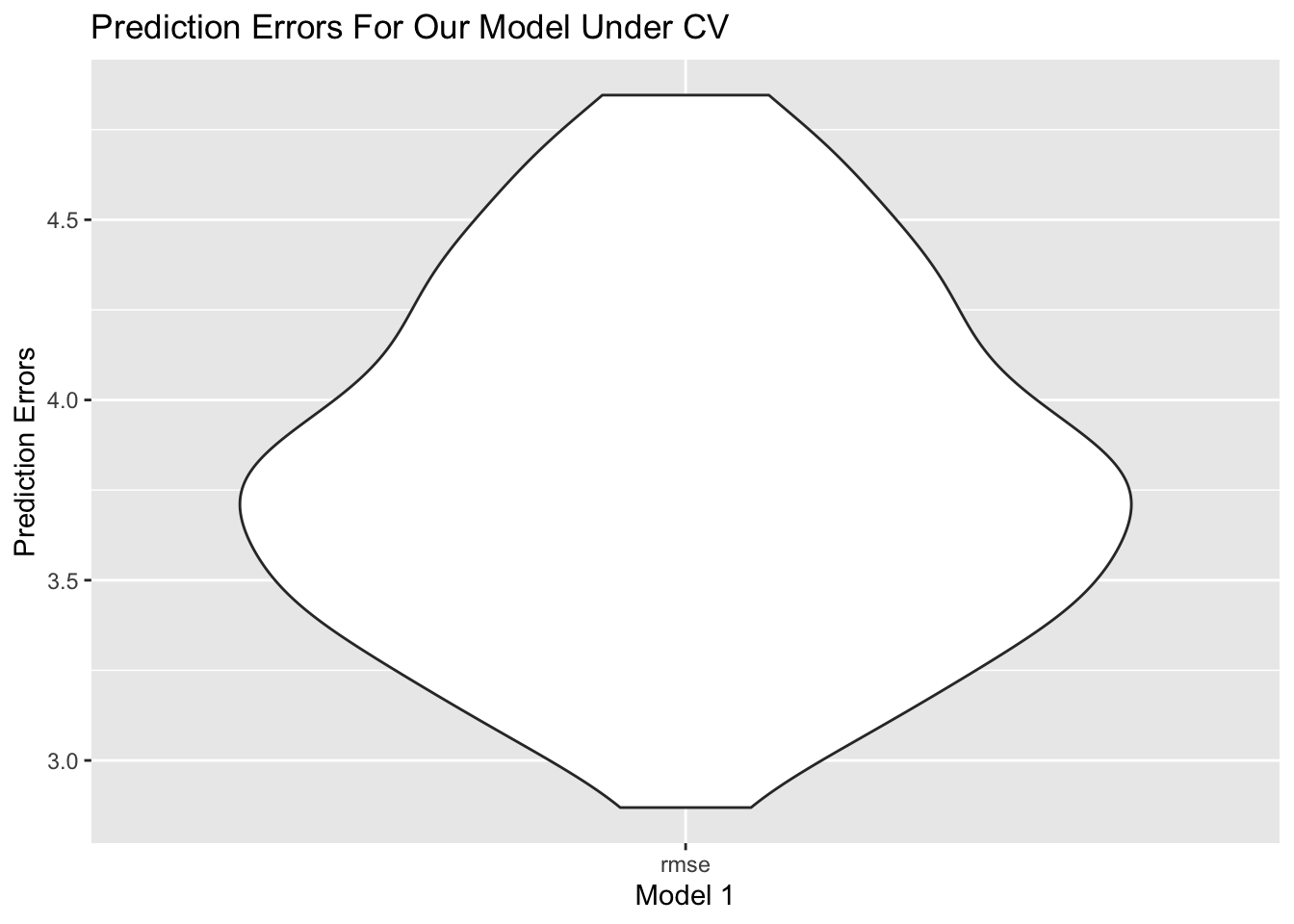
From the plot, RMSE is around 4.0, and spreads from 3.0 to 5.0, which is relatively a small and concentrated RMSE.
Prediction
The below graphs will show our prediction on Year 2016 data. Since we only have percent_w_in_lower_house data in year 2015, we will still use the same value for year 2016.
# predict on merged_data year 2016
data_2016 <-
  read_csv("data/Merged_expectation.csv") %>%
  filter(year == 2016) %>%
  select(une_life, alcohol, measles, basic_water, income_group) %>%
  bind_cols(data["percent_w_in_lower_house"]) %>%
  drop_na() %>%
  mutate(income_group = as.factor(income_group),
         income_group = relevel(income_group, ref = "Low income"))
prediction_2016 <- predict(m1, newdata = data_2016)
# draw ggplot1
ggp1 <- prediction_2016 %>%
  bind_cols(data_2016["une_life"])  %>%
  ggplot(aes(x = une_life, y = prediction_2016)) +
  geom_point() +
  geom_abline(intercept = 0, slope = 1, color = "red") +
  labs(
    title = "Prediction V.S. Actual Life Expectancy On Year 2016 In Original Dataset",
    x = "Actual Life Expectancy",
    y = "Prediction"
  )

# predict on imputed_data year 2016
data_2016_im <-
  read_csv("data/Imputed_expectation.csv") %>%
  filter(year == 2016) %>%
  select(une_life, alcohol, measles, basic_water, income_group) %>%
  bind_cols(data["percent_w_in_lower_house"]) %>%
  drop_na() %>%
  mutate(income_group = as.factor(income_group),
         income_group = relevel(income_group, ref = "Low income"))
prediction_2016_im <- predict(m1, newdata = data_2016_im)
# draw ggplot2
ggp2 <- prediction_2016_im %>%
  bind_cols(data_2016_im["une_life"])  %>%
  ggplot(aes(x = une_life, y = prediction_2016_im)) +
  geom_point() +
  geom_abline(intercept = 0, slope = 1, color = "red") +
  labs(
    title = "Prediction V.S. Actual Life Expectancy On Year 2016 In Imputed Dataset",
    x = "Actual Life Expectancy",
    y = "Prediction"
  )
ggp1 / ggp2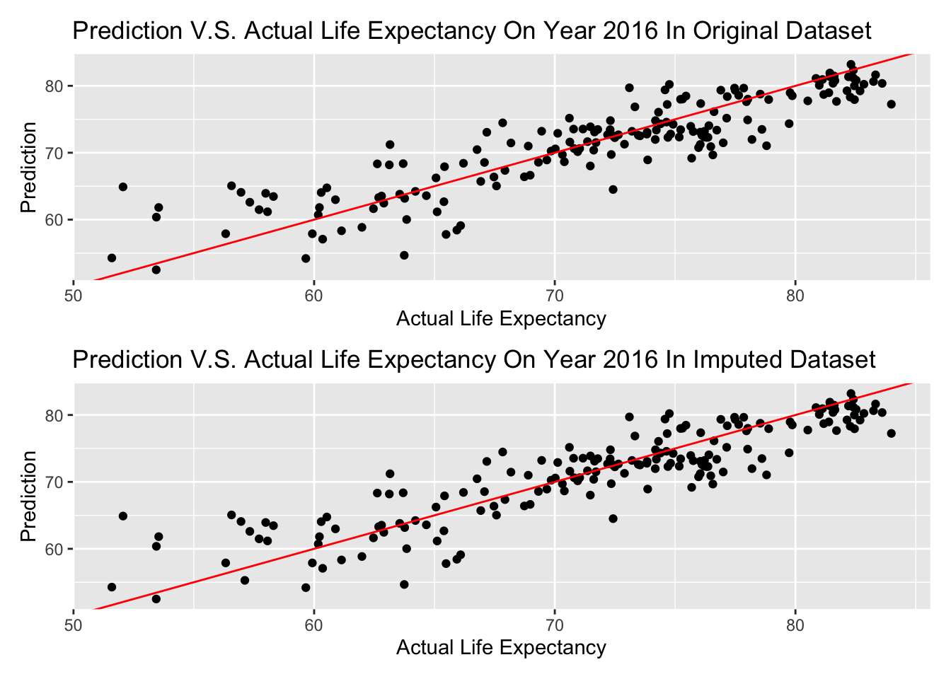
The graph above is shown that almost every prediction is in a + or - 5 years range, and there is no difference in imputed dataset and original dataset–possibly there is no data imputed on these variables of Year 2016.
If we consider a range in 3 years (+ or - 1.5 years) is a good prediction, lets see the percentage of predicted life expectancy in this range on Year 2016.
actual <- data_2016["une_life"]
percent <- sum(prediction_2016 >= actual - 1.5 & prediction_2016 <= actual + 1.5) / length(prediction_2016)
paste("The calculated result is ", round(percent, 3), ".")
## [1] "The calculated result is 0.369 ."Therefore, if we consider a range in 3 years (+ or - 1.5 years) is a good prediction, 0.369 of predicted life expectancy will be in this range on Year 2016.
Clustering
Clustering Analysis is an unsupervised method that cluster the countries of interest into groups in a high dimensional vector space, based on the information of predictors values, i.e. alcohol consumption, bmi value, measle vaccinations and etc in our analysis. Different from prediction, we focus on how countries are correlated with each other based on their predictors and more importantly, the optimal number of groups we can partition into based on all predictors. Based on the optimal number of groups, we can essentially impute our model using k mean clustering method. In our data cleaning, we impute our data using k=4. Here, we check whether k=4 is a good choice based on k mean clustering. The following code runs over k groups where k is between 1 to 10.
merged_data =
  read_csv("data/Merged_expectation.csv") %>%
  filter(year == 2015) %>%
  select(une_life,alcohol, bmi, measles, basic_water, che_gdp, une_gni, une_literacy, PM_value) %>%
  drop_na()

X_var =
  merged_data %>%
  select(alcohol, bmi, measles, basic_water, che_gdp, une_gni, une_literacy, PM_value)
Y_var =
outcomes = merged_data %>%
  select(une_life)


#Scale X variable
Scale_X = X_var %>%
  na.omit() %>%
  scale()


fviz_nbclust(Scale_X, kmeans, method = "silhouette") +
  theme_bw()
Here, we use silhouette method, which focus on how similar a point is within-cluster in comparison with other clusters paper. Based on the result, we discover that k =2,3 and 4 all has the highest sihouette width. k reaches its optimal value when k=4 and the optimal value coincide with our chosen k for k mean imputation value.
# get the kmean result and get the clusters
k_result =
  kmeans(x = X_var, centers = 4)

#Create the overall dataframe with combined Xvar Yvar and cluster
Allvalues =
  X_var %>%
  broom::augment(k_result, .) %>%
  cbind(Y_var,.)


# Plot predictor clusters against outcomes
ggplot(data = Allvalues, aes(x = une_gni, y = une_life, color = .cluster)) +
  geom_point(size=3) +
  labs(x = "GNI", y = "Life Expectancy", title = "Life expectancy vs GNI after clustered", color = "Cluster")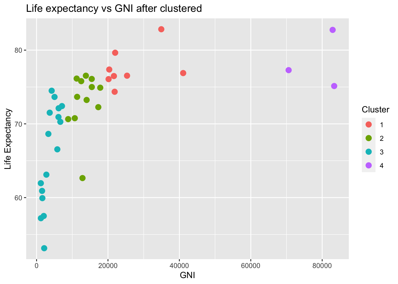
Although the algorithm is high dimensional, it is always better to visualize in a lower dimensional case when we only consider life expectancy and the predictor values. Here I choose GNI as an example. After clustering, we can clearly see that GNI with different clustered are clustered at different locations. This clustering may coincide with our previous classification with respect to different income group. High income group indicated by yellow color clearly has a relatively high life expectancy whereas low income group with low GNI value implied by the green group has a low life expectancy.
# Visualize cluster plot with reduction to two dimensions
fviz_cluster(k_result, data = X_var, palette = "Set2")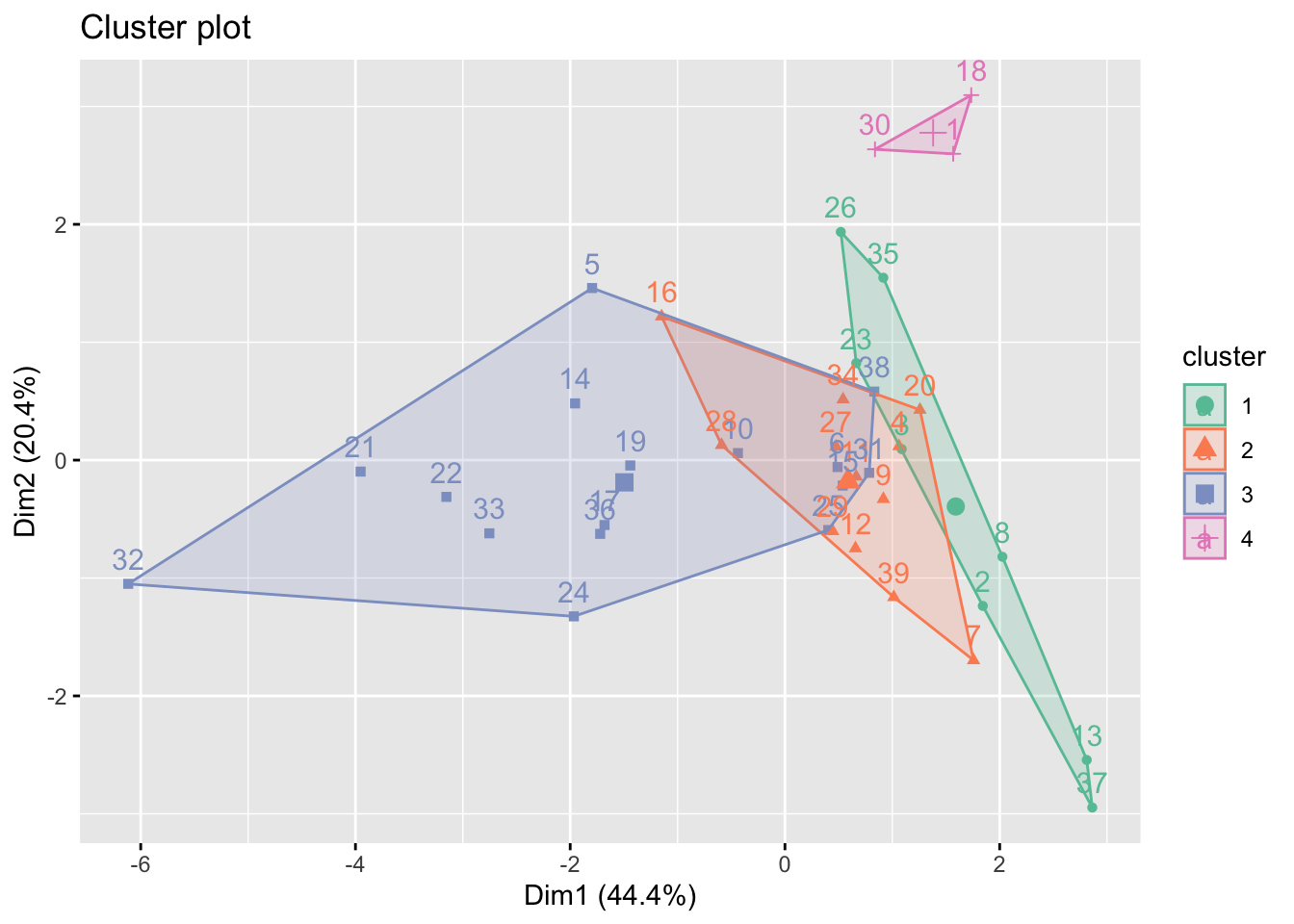
On the other hand, we plot based on the two highest variance explained dimension determined by principal component analysis (PCA). Most information are explained in the dimension 1 (44.4%) and dimension 2 (20.4%). As seen in the plot, only cluster 4 is clearly different from the other clusters. Cluster 1,2 and 3 are all intercorrelated with each other. This coincide with some of the time series plot in EDA part, i.e. number of doctors per 10,000 people and educational spend, which income groups overlapped with each other.
imputed_data =
  read_csv("data/Imputed_expectation.csv") %>%
  filter(year == 2015)

X_var_imp =
  imputed_data %>%
  select(alcohol, bmi, measles, basic_water, che_gdp, une_gni, une_literacy, PM_value)%>%
  na.omit() %>%
  scale()

Y_var_imp =
outcomes = imputed_data %>%
  select(une_life)

# get the kmean result and get the clusters
k_result_imp =
  kmeans(x = X_var_imp, centers = 4)

fviz_cluster(k_result_imp, data = X_var_imp, palette = "Set2")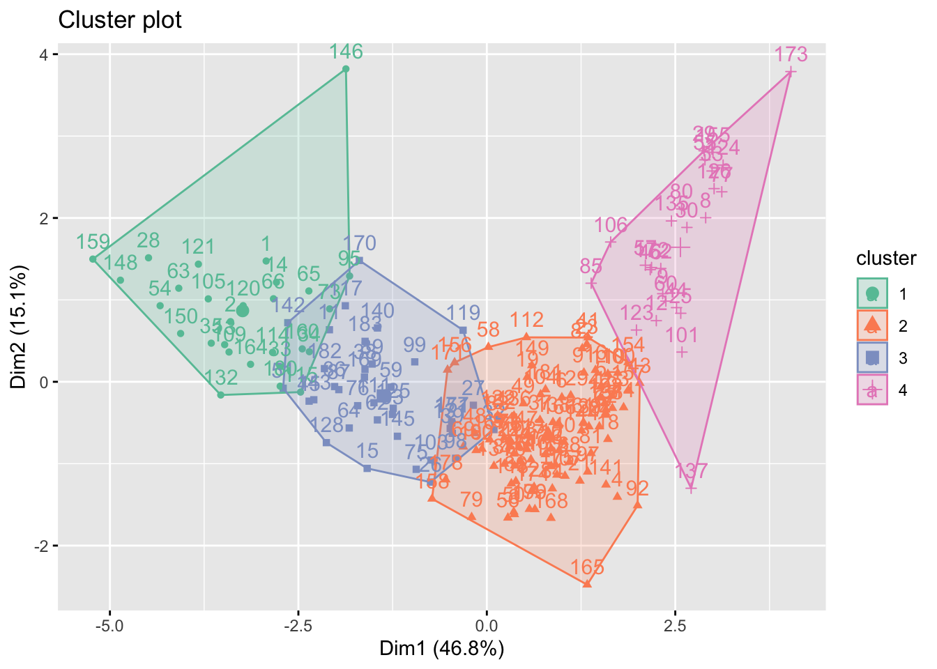
After imputation with k=4 mean clustering, the four groups are now separated from each other. This is reasonable because we impute with k=4 groups. Although the information may be biased, We can visualize that a high dimension 1 will lead to a high values in dimension 2. To our surprise, a low value in dimension 1 may also have a high value in dimension 2. This may because that some of the low income countries with low economic-related values may also have a high PM value.